RhinoCFD - Subscription
OverviewRhinoCFD is a general-purpose Computational Fluid Dynamics (CFD) plugin seamlessly integrated into the Rhino environment and powered by CHAM’s proven PHOENICS engine. It enables designers, engineers, and analysts to simulate how their models interact with air, water, and other fluids directly inside Rhino—eliminating the need to export geometry or switch between applications. This tight integration allows for rapid iteration, faster optimization, and a smoother, more intuitive workflow. With RhinoCFD, users can visualize flow patterns, pressure fields, heat transfer, and more, gaining essential insights early in the design process. Whether you're refining product performance, improving environmental behavior, or testing multiple design variables, RhinoCFD delivers reliable CFD capabilities within a familiar interface.
|
|
Features
RhinoCFD, which is compatible with Rhino 3D Versions 5, 6 and 7, adds the power of Computational Fluid Dynamics to the CAD environment. It allows Rhino3D users to undertake interactive CFD investigations of their CAD models operating under a multitude of flow conditions; and all without leaving the Rhinoceros environment.
RhinoCFD incorporates many of the unique, and best, features of PHOENICS.
- 'PARSOL' minimizes problems associated with handling complex geometries.
- Automatic Meshing avoids the necessity to spend hours optimizing meshes, and
- CONWIZ, the convergence wizard, greatly reduces the complexity of obtaining converged solutions.
Both steady-state and transient (time-dependent) scenarios can be considered, enabling users to extend the range of conditions applied to their models.
- Serial and parallel processing
- PARSOL cut-cell geometry detection simplifying the mesh generation process
- Numerous turbulence model options including RANS and LES
- Post-processing inbuilt in Rhino including isosurfaces, surface contours, vectors and streamlines
- Cartesian and Cylindrical Polar coordinate meshes
- In-program and online help
- Relational Data input without re-compiling
- Automatic convergence control
- Heat transfer between solids and fluids
- Radiation modelling
What's New
- New Post-Processing Panel - Expanded capabilities for post-processing results of a simulation:
- Redesign of the post-processing Viewer menu window – with new features and better organization.
- Variables (temperature, velocity, cell material, etc.) are displayed with full names in post-processing,
- Mathematical operations in post-processing can be performed on the data – e.g.: typing 0.5*Density*Velocity*Velocity” in the Scalar input box will calculate dynamic pressure in the flow.
- Standard notation added to scale; added feature to invert colors in post-processing; a grey-scale and
other color map options. - Improved performance of cutplane manipulation, including new faster vector drawing and improved shaders for coloring results.
- Added feature specular reflection to results objects (cutplanes, iso-surfaces, streamlines, etc.)
-
Improved foliage model, evaporation & mass transfer - The foliage object represents a group of trees or other vegetation. As trees and plants absorb heat and release water vapor, a pair of input boxes has been added to the Foliage object to allow entering the cooling rate in W/m3 and water-vapor release rate in kg/m3/s.
The ‘Heat source’ box should be set to the cooling power of the foliage (typically 250 W/m2) multiplied by the Leaf Area Density. The ‘Humidity source’ box (only available in Flair) should be set to the moisture source in kg/m2/s (of the order 810 g/m2/d), also multiplied by the Leaf Area Density. -
Automatic Time Step Calculation - An option in the ‘Time step settings’ dialog allows Earth to calculate the size of the time steps.
Dialog sets the size of time step 1. At the end of each time step the flow field is scanned for the largest Courant Number. The step size for the next step is adjusted to maintain ‘Target Courant Number’ within user-set limits. The run will stop when ‘Last step number’ steps have been performed, or time exceeds ‘Maximum total time’.
Current sweep number, time step number and time are written to any dumped solution files which enables restart runs to continue smoothly. This will benefit many transient cases where the timescale of the process changes during the calculation. This includes many VOF cases. - Option for outputting forces & moments per object as well as total - In addition to the pre-existing file containing the evolution of total force on all objects with time (or sweep), an additional file is output for each object participating in the force summation.
- New Thermal Boundary Condition on objects - Dialogs for setting boundary conditions on non-participating blockages (material 198) allow the setting of thermal and scalar sources on the outer surfaces of such objects.
-
Extensions to the Volume-Of-Fluid (VOF) method - VOF dialogues enable use of THINC, and setting of parameters required for temperature-dependent surface tension. All VOF methods can solve temperature-dependent cases, with proper treatment of the temperature in each phase and in any immersed solids.
Surface tension can be a linear function of temperature; the Langmuir equation of state can be used which includes a scalar as well as temperature. A constant static contact angle can be specified to model wall adhesion effects. -
Activation of Q-Criterion and Vorticity - The Main Menu – Output – Derived Variables panel allows activation of calculation and storage of the Q-criterion
and Vorticity.
Original: $2,879.00
-70%$2,879.00
$863.70
Description
OverviewRhinoCFD is a general-purpose Computational Fluid Dynamics (CFD) plugin seamlessly integrated into the Rhino environment and powered by CHAM’s proven PHOENICS engine. It enables designers, engineers, and analysts to simulate how their models interact with air, water, and other fluids directly inside Rhino—eliminating the need to export geometry or switch between applications. This tight integration allows for rapid iteration, faster optimization, and a smoother, more intuitive workflow. With RhinoCFD, users can visualize flow patterns, pressure fields, heat transfer, and more, gaining essential insights early in the design process. Whether you're refining product performance, improving environmental behavior, or testing multiple design variables, RhinoCFD delivers reliable CFD capabilities within a familiar interface.
|
|
Features
RhinoCFD, which is compatible with Rhino 3D Versions 5, 6 and 7, adds the power of Computational Fluid Dynamics to the CAD environment. It allows Rhino3D users to undertake interactive CFD investigations of their CAD models operating under a multitude of flow conditions; and all without leaving the Rhinoceros environment.
RhinoCFD incorporates many of the unique, and best, features of PHOENICS.
- 'PARSOL' minimizes problems associated with handling complex geometries.
- Automatic Meshing avoids the necessity to spend hours optimizing meshes, and
- CONWIZ, the convergence wizard, greatly reduces the complexity of obtaining converged solutions.
Both steady-state and transient (time-dependent) scenarios can be considered, enabling users to extend the range of conditions applied to their models.
- Serial and parallel processing
- PARSOL cut-cell geometry detection simplifying the mesh generation process
- Numerous turbulence model options including RANS and LES
- Post-processing inbuilt in Rhino including isosurfaces, surface contours, vectors and streamlines
- Cartesian and Cylindrical Polar coordinate meshes
- In-program and online help
- Relational Data input without re-compiling
- Automatic convergence control
- Heat transfer between solids and fluids
- Radiation modelling
What's New
- New Post-Processing Panel - Expanded capabilities for post-processing results of a simulation:
- Redesign of the post-processing Viewer menu window – with new features and better organization.
- Variables (temperature, velocity, cell material, etc.) are displayed with full names in post-processing,
- Mathematical operations in post-processing can be performed on the data – e.g.: typing 0.5*Density*Velocity*Velocity” in the Scalar input box will calculate dynamic pressure in the flow.
- Standard notation added to scale; added feature to invert colors in post-processing; a grey-scale and
other color map options. - Improved performance of cutplane manipulation, including new faster vector drawing and improved shaders for coloring results.
- Added feature specular reflection to results objects (cutplanes, iso-surfaces, streamlines, etc.)
-
Improved foliage model, evaporation & mass transfer - The foliage object represents a group of trees or other vegetation. As trees and plants absorb heat and release water vapor, a pair of input boxes has been added to the Foliage object to allow entering the cooling rate in W/m3 and water-vapor release rate in kg/m3/s.
The ‘Heat source’ box should be set to the cooling power of the foliage (typically 250 W/m2) multiplied by the Leaf Area Density. The ‘Humidity source’ box (only available in Flair) should be set to the moisture source in kg/m2/s (of the order 810 g/m2/d), also multiplied by the Leaf Area Density. -
Automatic Time Step Calculation - An option in the ‘Time step settings’ dialog allows Earth to calculate the size of the time steps.
Dialog sets the size of time step 1. At the end of each time step the flow field is scanned for the largest Courant Number. The step size for the next step is adjusted to maintain ‘Target Courant Number’ within user-set limits. The run will stop when ‘Last step number’ steps have been performed, or time exceeds ‘Maximum total time’.
Current sweep number, time step number and time are written to any dumped solution files which enables restart runs to continue smoothly. This will benefit many transient cases where the timescale of the process changes during the calculation. This includes many VOF cases. - Option for outputting forces & moments per object as well as total - In addition to the pre-existing file containing the evolution of total force on all objects with time (or sweep), an additional file is output for each object participating in the force summation.
- New Thermal Boundary Condition on objects - Dialogs for setting boundary conditions on non-participating blockages (material 198) allow the setting of thermal and scalar sources on the outer surfaces of such objects.
-
Extensions to the Volume-Of-Fluid (VOF) method - VOF dialogues enable use of THINC, and setting of parameters required for temperature-dependent surface tension. All VOF methods can solve temperature-dependent cases, with proper treatment of the temperature in each phase and in any immersed solids.
Surface tension can be a linear function of temperature; the Langmuir equation of state can be used which includes a scalar as well as temperature. A constant static contact angle can be specified to model wall adhesion effects. -
Activation of Q-Criterion and Vorticity - The Main Menu – Output – Derived Variables panel allows activation of calculation and storage of the Q-criterion
and Vorticity.